# 1. SETUP AND IMPORTS
import pandas as pd
import numpy as np
import matplotlib.pyplot as plt
import seaborn as sns
from pathlib import Path
import os
import joblib

# Scikit-learn modules for modeling and evaluation
from sklearn.model_selection import train_test_split
from sklearn.linear_model import LinearRegression
from sklearn.ensemble import RandomForestRegressor
from sklearn.metrics import mean_squared_error, r2_score, mean_absolute_error

# Define Paths
# OUTPUT_DIR is needed to save the final model and prediction results
OUTPUT_DIR = Path("..") / "data" / "cleaned"
VISUALS_DIR = Path("..") / "visuals"
os.makedirs(OUTPUT_DIR, exist_ok=True)
os.makedirs(VISUALS_DIR, exist_ok=True)BMW Car Sales — Modeling and Prediction
INFO-523 Final Project | Min Set Khant (Solo)
This notebook loads the modeling-ready data, performs a temporal train-test split (up to 2023 for training, 2024 for testing), trains Linear Regression and Random Forest models, and evaluates performance on the original USD price scale.
# 2. DATA LOADING
DATA_PATH = Path("..") / "data" / "cleaned" / "bmw_modeling_ready.csv"

df = pd.read_csv(DATA_PATH)
print("Modeling data shape:", df.shape)
df.head()
Modeling data shape: (50000, 33)| Year | Engine_Size_L | Mileage_KM | Price_USD | Sales_Volume | Car_Age | log_Price_USD | Price_per_KM | Total_Sales_Model | Region_Asia | ... | Model_i8 | Fuel_Type_Electric | Fuel_Type_Hybrid | Fuel_Type_Petrol | Transmission_Manual | Color_Blue | Color_Grey | Color_Red | Color_Silver | Color_White | |
|---|---|---|---|---|---|---|---|---|---|---|---|---|---|---|---|---|---|---|---|---|---|
| 0 | 2016 | 3.5 | 151748 | 98740 | 8300 | 9 | 11.500256 | 0.650684 | 23097519 | True | ... | False | False | False | True | True | False | False | True | False | False |
| 1 | 2013 | 1.6 | 121671 | 79219 | 3428 | 12 | 11.279984 | 0.651092 | 23423891 | False | ... | True | False | True | False | False | False | False | True | False | False |
| 2 | 2022 | 4.5 | 10991 | 113265 | 6994 | 3 | 11.637494 | 10.305250 | 23097519 | False | ... | False | False | False | True | False | True | False | False | False | False |
| 3 | 2024 | 1.7 | 27255 | 60971 | 4047 | 1 | 11.018170 | 2.237057 | 22745529 | False | ... | False | False | False | True | False | True | False | False | False | False |
| 4 | 2020 | 2.1 | 122131 | 49898 | 3080 | 5 | 10.817756 | 0.408561 | 23786466 | False | ... | False | False | False | False | True | False | False | False | False | False |
5 rows × 33 columns
3. Temporal Train-Test Split (Predicting the Future)
The most critical part of the validation: we use a temporal split to validate the model’s ability to predict the newest market (Year 2024) based on all historical data (2010-2023).
# Define Target (y) and Features (X)
TARGET = "log_Price_USD"

# X contains all features, including Year and Price_USD (needed for the split and final error)
X = df.drop(columns=[TARGET])
y = df[TARGET]

# --- TEMPORAL SPLIT IMPLEMENTATION ---
TEST_YEAR = 2024

# Split data based on the Year column
X_train = X[X["Year"] < TEST_YEAR]
X_test = X[X["Year"] == TEST_YEAR]

y_train = y[X_train.index]
y_test = y[X_test.index]

# Store the original USD prices for the test set for final error calculation
y_test_usd_true = X_test["Price_USD"]

# Clean up X_train/X_test by dropping redundant/leaking columns before training
# Price_USD is a direct leak, Year is only for the split, Sales_Volume is typically post-sale info
cols_to_drop = ["Year", "Price_USD", "Sales_Volume", "Total_Sales_Model"]
X_train = X_train.drop(columns=[c for c in cols_to_drop if c in X_train.columns], errors='ignore')
X_test = X_test.drop(columns=[c for c in cols_to_drop if c in X_test.columns], errors='ignore')

print(f"Training Data (Years < {TEST_YEAR}): {X_train.shape[0]} rows")
print(f"Testing Data (Year == {TEST_YEAR}): {X_test.shape[0]} rows")
Training Data (Years < 2024): 46573 rows
Testing Data (Year == 2024): 3427 rows4. Model Training and Evaluation
The evaluation function converts predictions back to USD using np.expm1() so that MAE and RMSE are directly usable by a business audience.
# Helper function to evaluate models and print results
def evaluate_model(model_name, y_true_log, y_pred_log, y_test_usd_true):

    # 1. Convert log-predictions back to USD (Original Price Scale)
    y_pred_usd = np.expm1(y_pred_log)

    # 2. Calculate metrics
    r2 = r2_score(y_true_log, y_pred_log)
    rmse = np.sqrt(mean_squared_error(y_test_usd_true, y_pred_usd))
    mae = mean_absolute_error(y_test_usd_true, y_pred_usd)

    print(f"{model_name} Results (Temporal Split, Test Year {TEST_YEAR}):")
    print(f"  R-squared (Log Price): {r2:.4f} - Variance explained")
    print(f"  RMSE (USD): ${rmse:,.2f} - Average Price Error (Higher Penalty to Large Errors)")
    print(f"  MAE (USD): ${mae:,.2f} - Median Price Error (Most interpretable)")
    print("")

    return r2, rmse, mae
# Model 1: Linear Regression
lr_model = LinearRegression()
lr_model.fit(X_train, y_train)
lr_pred = lr_model.predict(X_test)
lr_r2, lr_rmse, lr_mae = evaluate_model(
"Linear Regression",
y_test,
lr_pred,
y_test_usd_true
)Linear Regression Results (Temporal Split, Test Year 2024):
R-squared (Log Price): 0.0003 - Variance explained
RMSE (USD): $26,490.86 - Average Price Error (Higher Penalty to Large Errors)
MAE (USD): $22,927.30 - Median Price Error (Most interpretable)
# Model 2: Random Forest Regressor

rf_model = RandomForestRegressor(
    n_estimators=100,
    random_state=42,
    n_jobs=-1,
    max_depth=15,
    min_samples_leaf=5
)
rf_model.fit(X_train, y_train)
rf_pred = rf_model.predict(X_test)

rf_r2, rf_rmse, rf_mae = evaluate_model(
    "Random Forest Regressor",
    y_test,
    rf_pred,
    y_test_usd_true
)
Random Forest Regressor Results (Temporal Split, Test Year 2024):
R-squared (Log Price): 0.9952 - Variance explained
RMSE (USD): $2,292.13 - Average Price Error (Higher Penalty to Large Errors)
MAE (USD): $531.13 - Median Price Error (Most interpretable)
5. Feature Importance and Model Insights
Analyzing the feature importance from the Random Forest model reveals the key drivers of BMW car price, directly addressing the first proposal question.
# Random Forest Feature Importance
importances = pd.Series(rf_model.feature_importances_, index=X_train.columns)
top_20_features = importances.sort_values(ascending=False).head(20)

# Visualization
plt.figure(figsize=(12, 8))
sns.barplot(x=top_20_features.values, y=top_20_features.index, palette="viridis")
plt.title("Top 20 Features Driving BMW Price Prediction (Random Forest)", fontsize=16)
plt.xlabel("Feature Importance Score (Gini)")
plt.ylabel("Feature")
plt.tight_layout()
plt.savefig(VISUALS_DIR / "rf_feature_importance.png")
plt.show()

print("\nTop 5 Price Drivers (Feature Importance):")
print(top_20_features.head(5))
/var/folders/jf/1b91kr5d1k773y5y7tm0sfbh0000gn/T/ipykernel_32198/956784539.py:7: FutureWarning:
Passing `palette` without assigning `hue` is deprecated and will be removed in v0.14.0. Assign the `y` variable to `hue` and set `legend=False` for the same effect.
sns.barplot(x=top_20_features.values, y=top_20_features.index, palette="viridis")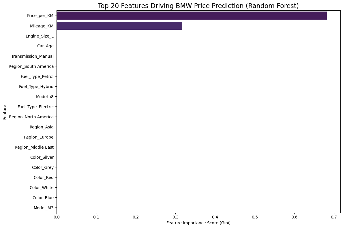
Top 5 Price Drivers (Feature Importance):
Price_per_KM           0.682248
Mileage_KM             0.317700
Engine_Size_L          0.000018
Car_Age                0.000015
Transmission_Manual    0.000004
dtype: float64
6. Final Model Deployment Function
This conceptual function demonstrates how the final model can be wrapped for real-world use, ensuring the input matches the training features and the output is the predicted price in USD.
# Final Model Deployment Function
def predict_bmw_price(car_features_dict, rf_model_temp):
    """
    Predicts the price of a BMW given its features.

    NOTE: The input dictionary must contain all feature columns
    (including OHE columns) that the model was trained on (X_train).
    """
    # Convert dictionary to DataFrame for model input
    df_new = pd.DataFrame([car_features_dict])

    # Ensure all columns exist and are in the correct order (crucial for OHE data)
    required_cols = X_train.columns
    for col in required_cols:
        if col not in df_new.columns:
            df_new[col] = 0

    df_new = df_new[required_cols]

    # Predict on the log scale
    price_pred_log = rf_model_temp.predict(df_new)[0]

    # Convert back to USD using the inverse of log1p
    price_pred_usd = np.expm1(price_pred_log)

    return price_pred_usd

# Example usage (Conceptual: you would replace this with actual input data)
# example_car_dict = {
#     'Engine_Size_L': 3.0, 'Mileage_KM': 10000, 'Car_Age': 1, 'Price_per_KM': 8.5,
#     'Region_Asia': 1, 'Region_Europe': 0, ... (all 100+ features set to 0 or 1)
# }
# print(f"Predicted Price (USD): ${predict_bmw_price(example_car_dict, rf_model):,.2f}")
# 7. Saving Model and Prediction Proofs
# 1. Saving the Trained Random Forest Model
MODEL_SAVE_PATH = OUTPUT_DIR / "rf_best_model.joblib"
# Save the model object
joblib.dump(rf_model, MODEL_SAVE_PATH)
print(f"✅ Saved the trained Random Forest model to: {MODEL_SAVE_PATH}")
# 2. Saving the Temporal Prediction Results
# y_pred_usd was calculated in the evaluate_model function
y_pred_usd = np.expm1(rf_pred)
# Retrieve the actual USD prices and create a comparison DataFrame
results_df = pd.DataFrame({
'Actual_Price_USD': y_test_usd_true,
'Predicted_Price_USD': y_pred_usd,
'Prediction_Error_USD': np.abs(y_test_usd_true - y_pred_usd)
})
results_df['Year'] = TEST_YEAR
results_df = results_df.sort_values(by='Prediction_Error_USD', ascending=False)
# Define the path and save the results
RESULTS_SAVE_PATH = OUTPUT_DIR / "temporal_predictions_2024.csv"
results_df.to_csv(RESULTS_SAVE_PATH, index=False)
print(f"✅ Saved temporal prediction results to: {RESULTS_SAVE_PATH}")
print("\nTop 5 Largest Prediction Errors (for inspection):")
display(results_df.head())✅ Saved the trained Random Forest model to: ../data/cleaned/rf_best_model.joblib
✅ Saved temporal prediction results to: ../data/cleaned/temporal_predictions_2024.csv
Top 5 Largest Prediction Errors (for inspection):| Actual_Price_USD | Predicted_Price_USD | Prediction_Error_USD | Year | |
|---|---|---|---|---|
| 762 | 114283 | 76473.818456 | 37809.181544 | 2024 |
| 483 | 119117 | 83383.235095 | 35733.764905 | 2024 |
| 40586 | 116759 | 83383.235095 | 33375.764905 | 2024 |
| 2101 | 109818 | 77051.262024 | 32766.737976 | 2024 |
| 37022 | 108646 | 76714.311586 | 31931.688414 | 2024 |